Diving Into Temporal Convolutional Networks
One important area of neural network applications is sequence modeling, or the process of capturing temporal structures in data for purposes of time series prediction, classification, and generation. Sequence modeling spans tasks such as speech recognition, sentiment classification, and machine translation. We usually equate sequence modeling with recurrent models–specifically recurrent neural networks such as Long Short Term Memory Networks (LSTMs) or Gated Recurrent Units (GRUs). The textbook used in my Neural Nets course even titles the chapter on sequence modeling “Sequence Modeling: Recurrent and Recursive Nets”.
However, recent results challenge the notion that recurrent networks provide the best performance on sequence modeling tasks. Some convolutional architectures have actually demonstrated state-of-the art performance. A recent comparison of a generic convolutional architecture against contemporary recurrent models demonstrated superior performance of a convolutional-based design across a range of sequence modeling tasks.
Sequence modeling can be described as finding a function \(f\) which maps a given input sequence \(x_{0},x_{1},..., x_{n}\) to a corresponding output sequence \(y_{0},y_{1},..., y_{n}\) for each time \(t\) such that \(f( x_{0} ,x_{1} ,...,x_{t}) = y_{0} ,y_{1} ,...,y_{t}\). Here, the function \(f\) is causal in that it doesn’t depend on any future inputs \(x_{t+1}\). A neural network solving a sequence modeling task aims to minimize the loss \(L(y_{0},y_{1},..., y_{t}, f(x_{0},x_{1},...,x_{t})))\) between the predicted and actual sequence outputs. The specific loss function varies depending on the task being learned.
Temporal Convolutional Networks
A TCN describes a general convolutional network architecture which takes a sequence of arbitrary length and maps it to an output sequence of the same length. The network architecture of a TCN is an extension of a 1D CNN, in which a series of 1D convolutional layers are stacked on one another. A vanilla 1D convolutional layer can be written as:
\[F(\boldsymbol{x}\mathbf{_{t}}) \ =\ \mathbf{(}\boldsymbol{x} \ \circledast \ \boldsymbol{f})( t) \ =\ \sum ^{k}_{j=-k}\boldsymbol{f}[ j]\boldsymbol{x}[ t-j]\]where \(x\) is the input sequence and \(f\) is a convolutional filter of size \(2k+1\) applied at time \(t\).
Causal Convolutions
This basic convolution operation relies on a causal input and filter, which is undesirable for sequence modeling tasks since the convolution operation relies on future time points. A causal version of a 1D convolution can be written as:
\[F(\boldsymbol{x}\mathbf{_{t}}) \ =\ \mathbf{(}\boldsymbol{x} \ \circledast \ \boldsymbol{f})( t) \ =\ \sum ^{k}_{j=0}\boldsymbol{f}[ j]\boldsymbol{x}[ t-j]\]where \(k\) is the size of the filter being learned. Note that this vanilla 1D convolutional layer takes a length \(n\) sequence as input and returns a length \(n-k+1\) sequence. Concatenating zero padding of length \(k-1\) at the beginning of the sequence maintains an equivalent output length, while also allowing for an easy implementation of causal convolutions by running a standard, non-causal convolution over the \(k-1\) shifted input sequence. Stacking multiple 1D convolutions allows for a simple 1D CNN structure depicted below:
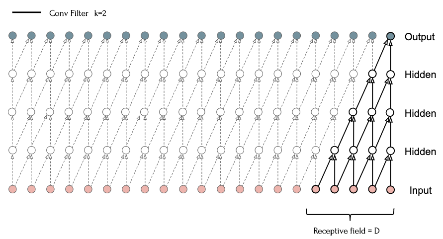
Here, four 1D convolutional layers \((k=2)\) are stacked such that the output at each time \(t\) relies on the previous four inputs. This structure, similar to that proposed in the WaveNet paper, has a receptive field that scales linearly with depth. This linear scaling requires very deep networks in order to capture the history required for many sequence modeling tasks. Dilated convolutions are one solution to this problem, as they result in an exponentially larger receptive field.
Dilated Convolutions
A dilated convolution modifies the causal convolution by a dilation factor \(d\) such that:
\[F(\boldsymbol{x}\mathbf{_{t}}) \ =\ \mathbf{(}\boldsymbol{x} \ \circledast _{d} \ \boldsymbol{f})( t) \ =\ \sum ^{k}_{j=0}\boldsymbol{f}[ j]\boldsymbol{x}[ t-( d\ *\ j)]\]By expanding the dilation factor for each layer \(i\) such that \(d_{i} = 2_{i}-1\), exponentially larger receptive fields can be captured as depth increases. For a 1D convolution block of depth \(D\), this expands the receptive field to \(2^{D-1}*k\), allowing for a very large effective history as a function of depth.
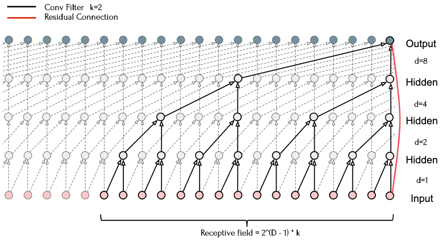
The above diagram shows such a generic residual module with four layers (\(k\)=2), and a residual connection from the input directly to the output layer. This reveals how dilations can be used to sample the entire input sequence, while also building a larger effective history.
Residual Connections
As network depth increases, it can become more difficult to back-propagate error to earlier layers, resulting in challenges during training. Residual blocks introduce a connection bus allowing for quicker learning.
\[o = Activation(\mathbf{x} \ +\ F(\mathbf{x}))\]Where the new output \(o\) is the sum of the blocks input \(x\) and a series of transformations \(f\) on the input. In this case the transformations \(f\) are defined by the operations in the 1D convolutional layers. Dilated convolutions and residual connections can then be combined to form a generic residual model which can be used to form larger architectures.
The figure below shows the same generic residual module stacked to form multiple layers, further expanding the receptive field while still stabilizing training using the residual connection.
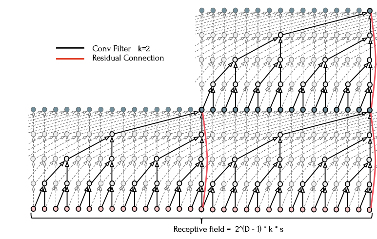
These residual modules also contain commonly found neural network components such as a nonlinearity applied after the convolutional pass, weight normalization, and dropout. Once residual stacks are added to the architecture, the full receptive field of the TCN of depth \(D\), kernel size \(k\), and \(s\) residual blocks can be calculated as:
\[RF = 2^{D-1} \ *\ k\ *\ s\]Now that we have a full temporal convolutional network, the question arises–how does the architectural composition affect performance? If the receptive field is smaller than the temporal domain we need to capture, performance will suffer, as the network isn’t able to retain information far enough into the past. However, we can achieve the same receptive field using a different composition of kernel size, residual blocks, and stacks of 1D convolutions. Other meta-properties of the network may also impact performance; larger depths may make training more difficult, more weights may contribute to training performance while also causing overfitting.
It is also interesting to explore whether certain architectural properties are universally advantageous, or the optimal configuration varies depending on the sequence modeling task we are solving. Image-based CNNs can be easily extended to leverage information from similar domains (transfer learning). Different receptive fields and optimal configurations across sequence modeling tasks would indicate that transfer learning with TCNs could be more challenging.
Experiments
In order to explore these questions, I set up experiments using the elegant keras TCN implementation. I based experiments on three sequence modeling tasks all supported out-of-the-box with this implementation. The task description images included below are also courtesy of the library.
Adding Task
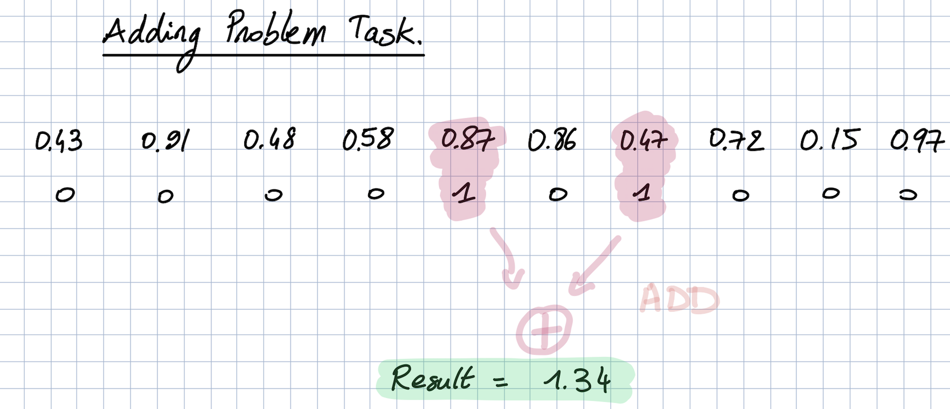
The adding task is a synthetic regression task in which the goal is to predict the sum of two random numbers from an array of floating point numbers. A second Boolean array (true at these two values, false everywhere else) indicates which numbers should be added.
Copy Memory Task
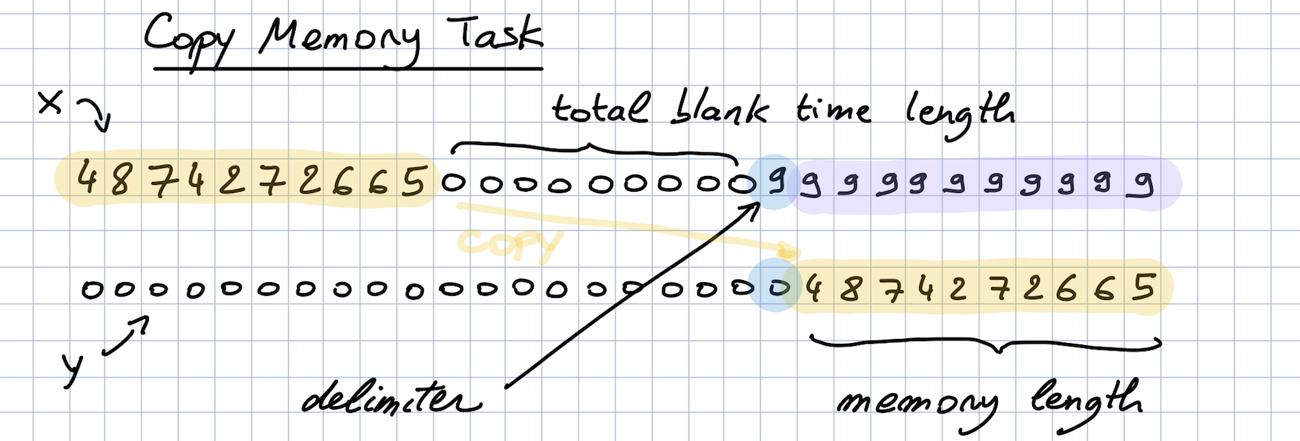
The copy memory task is a synthetic classification task. Here, the point is to copy a buffer of numbers presented at the beginning of the sequence after a flag value is encountered at the end of the sequence. This task is ideal for examining retention of information from the distant past, as the sequence length can easily be changed by varying the time before the flag value is encountered.
Sequential MNIST Task
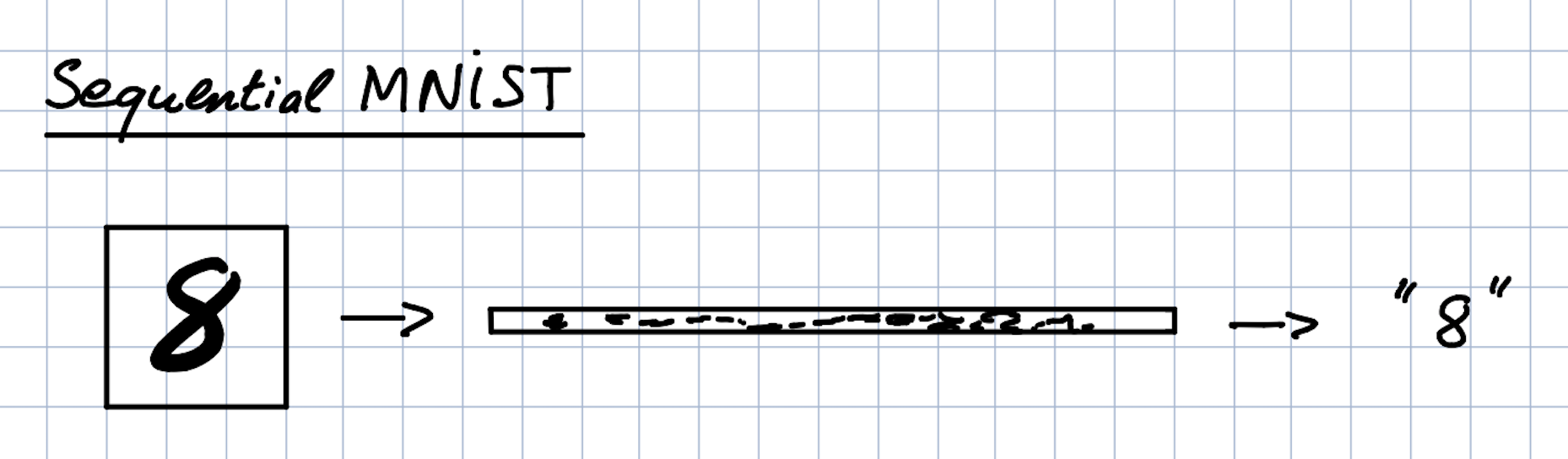
The sequential MNIST task is a variation of the MINST task (classifying a written digits), except that pixels are presented sequentially as opposed to 2D form.
Across experiments, I used Adam with a constant learning rate of \(1e^{-4}\), 20 convolutional filters at each layer, and no dropout or weight norm. Models were also trained for 100 epochs each.
The simplest way to examine the contribution of each architectural parameter is to vary it in isolation. So, I set up an experiment which varied the kernel size, number of dilated layers, and residual stacks while keeping the others fixed. This test does have a drawback. Based on the receptive field equation above, we see that the receptive field size (and number of overall weights) will increase as we increase each of these parameters. Therefore, I also set up a second experiment which fixes the receptive field by varying two parameters in conjunction–as one parameter increases to expand the receptive field size, the other decreases to accommodate. This gives us three permutations of parameter combinations in the second experiment:
- Kernel size vs. number of dilations
- Kernel size vs. number of residual blocks
- Number of dilations vs. number of residual blocks
Note that while this does control for receptive field size, some models will still contain more parameters than others. The performance results of the architectures we get using this configuration are below.
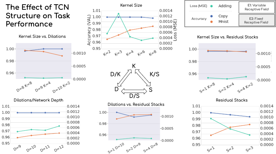
Here, the white graphs show the variable receptive field experiment, while the grey ones show the fixed receptive field experiment. The left axis on each chart describes validation classification accuracy for the s-MNIST and copy memory task, while the right axis shows validation MSE achieved in the adding task. The triangular arrangement underscores the two experiments’ setup–the vertices show the effect of changing only one parameter, while the edges show varying parameters in conjunction.
The first thing that we notice is that the TCN is performing well across all tasks, and is relatively robust to changes in the architecture. However, we do see the models responding to changes in composition.
While looking at the adding task results, we see that although varying each parameter in isolation appears to impact performance noticeably, when we control for the receptive field size, this effect disappears and performance remains constant. We see roughly the same story with the copy memory task–variability introduced by varying a single parameter tends to disappear once the receptive field size is controlled for. There do seem to be some settings that perform worse across experiments, for example having a smaller number of dilated layers (D=8 condition). The s-MNIST task shows sensitivities which remain even after controlling for the receptive field size; for example, more dilations do not compensate for a small kernel size. This indicates the TCN trained to perform s-MNIST performs more optimally with a larger kernel size.
We also see concrete evidence that there is no one-size-fits-all architecture for sequence modeling tasks. Even after controlling for receptive field size, the two classification tasks respond differently with various combinations of kernel size vs. dilations, and dilations vs. residual stacks.
Although this graph begins to paint a picture of how the model is responding to different hyperparameters, it is still difficult to see how other meta-factors such as the number of trainable parameters and depth are influencing performance. By plotting results as a function of trainable parameters, depth, and receptive field size, we can better understand what is going on.
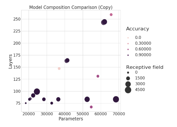
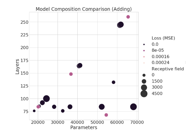
Below, the two axes show the number of layers and trainable parameters, while the size of each bubble reflects the receptive field length. The hue of the bubble shows the corresponding performance. Not only does this figure tell us an interesting story about how the model is responding to these three factors, but we also see visual connections between architecture parameters.
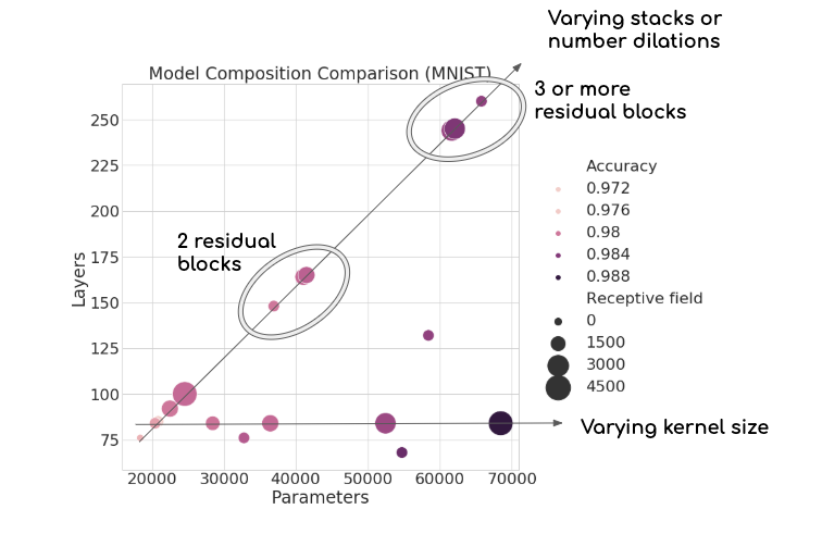
The TCN performing s-MNIST shows that the most important factor (for this dataset) is actually the number of trainable parameters. Performance is scaling linearly as we add more weights, regardless of receptive field size. We also see that receptive field size isn’t all that matters–models with comparatively small receptive fields and few weights can still out-perform deeper or larger networks. We also observe two axes of architectures, which make since given our intuition regarding how the TCN is structured.
For example, increasing the kernel size won’t increase the depth of the network, but will increase the number of weights and the receptive field size. This gives the flat horizontal axes. Secondly, we see another axis moving linearly upwards. This axis reflects the relationship between increasing layers and parameters in the network. We also see clusters organized according to how many stacks the network consists of: adding another stack or two greatly bolsters the overall network depth.
The two synthetic tasks tended to perform robustly overall, with the exception of a few configurations:
In a final experiment, I changed the length of the sequence to be retained in the copy memory task while keeping the architecture (and therefore receptive field) fixed. I expected solid performance until the sequence length exceeded the receptive field size, at which point I suspected performance would tank.
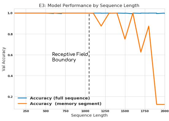
Sure enough, we see high accuracy until the point where the receptive field was exceeded, followed by diminishing results. Interestingly, however, the model could still perform the task (to some degree) until the sequence length was nearly twice the length of the network’s receptive field. Plotting the performance of only the last 10 digits in the memory segment makes this effect more clear. This slowly deteriorating performanc could be because this task is arbitrary–perhaps with a more complicated memory payload, performance would indeed deteriorate immediately.
Takeaways
Overall, we see results that mirror what TCN’s have been showing so far: good results robust to a variety contexts and configurations. In some tasks, adding more weights will consistently help achieve the desired accuracy, while in others, getting the architectural configuration correct is vital. Different sequence modeling tasks respond to model changes in different ways, but the \(k\)=8 configuration in the bottom right plot does perform well across tasks. This could simply be because this configuration has the most trainable parameters, however.
There you have it! An introduction and some experiments exploring Temporal Convolutional Networks. Curious to learn more or apply them to a sequence learning problem? Clone down keras TCN implementation and dive in.