How to Decode Mental States With a Commercial EEG Headband
Wearable devices are becoming more and more common, giving us access to an unprecedented amount of real-time physiological data. These wearables are useful for tracking things like activity levels and exercise, but we can also use them for much more powerful applications.
Take for example wearable electroencephalography (EEG) headbands. These devices give direct access to a high level overview of the brain’s electrical activity–an “outside of the ballpark” view of what is going on in the mind. Though we might not be able to decode thoughts with a few dry electrodes, we can get a sense of global states such relaxation, alertness, or fatigue. What if we could take it one step further and create environments which respond interactively to how we are feeling? This is similar to the paradigm is often referred to as neurofeedback, which has many potential applications.
Today we will use a Muse headband–one of the most common and easily accessible EEG headsets–to create two types of interactive environments. I will show you:
- How to decode mental signals recorded using the Muse headband
- Different ways of making use of these signals in an interactive environment
The environment aspect of this can get complicated–but I will show a few examples of how the signals can be applied without diving into environments’ implementation details.
A basic mental state decoding algorithm
Connecting with the MUSE
So you have access to a Muse headband? Great! The first thing we need to do is get a connection up and running. The exact process of achieving this will depend on the version of headband that you have. If you have a 2014 Muse headband, you can connect this device to your laptop via an OSC stream, which is supported by Muse out of the box . If you have a Muse 2016 headband, this gets more tricky, since this device connects using Bluetooth low energy, which isn’t supported directly by most laptop computers. MuseLSL is a good option for connecting with a Muse 2016 headband. Note that the authors also include a nifty neurofeedback script that will implement most of what I talk about here.
Regardless of the method you use, I’ll assume that you now have a Python script reading in values that the headband emits in real time, either using MuseLSL with the 2016 headband or a sample script provided by the Muse developers for the 2014 headband (sorry, I haven’t worked with Muse 2 yet, so don’t have any instructions for that device).
Decoding signals from EEG
Now that we have real time EEG signals, there are a few different options for how to decode them. One option is to build out a supervised machine learning model and use that to classify mental states categorically or predict the value within a continuous range. Though this could work, there are a few reasons why it is a pain:
-
Labels. At the end of the day, any supervised model will need ground truth labels–and lots of them–to build a mapping from the electrical activity to the higher-level mental activity. Having lots of time-locked and continuous labels can be tricky and a lot of work. Now, you may think, there are plenty of datasets I can already use to train a model, why not use one of those?
-
Variability. When it comes to complex signals like EEG, there is a large amount of variability depending on the person and session, meaning that it is hard to achieve high accuracy on a new person or session if training does not match that context.
If you can overcome both of these challenges, you may get stellar performance and an awesome decoding algorithm. Alas, there are other methods that require much less upfront work.
Frequency-based decoding
You may remember me mention that EEG is based on electrical activity in the brain–electrical activity which consists of many different frequencies combined together. It turns out that different frequencies are indicative of different mental phenomena. Not only is this frequency mapping robust across people, it is also consistent across time: a perfect phenomenon to use in our basic mental state decoding algorithm.
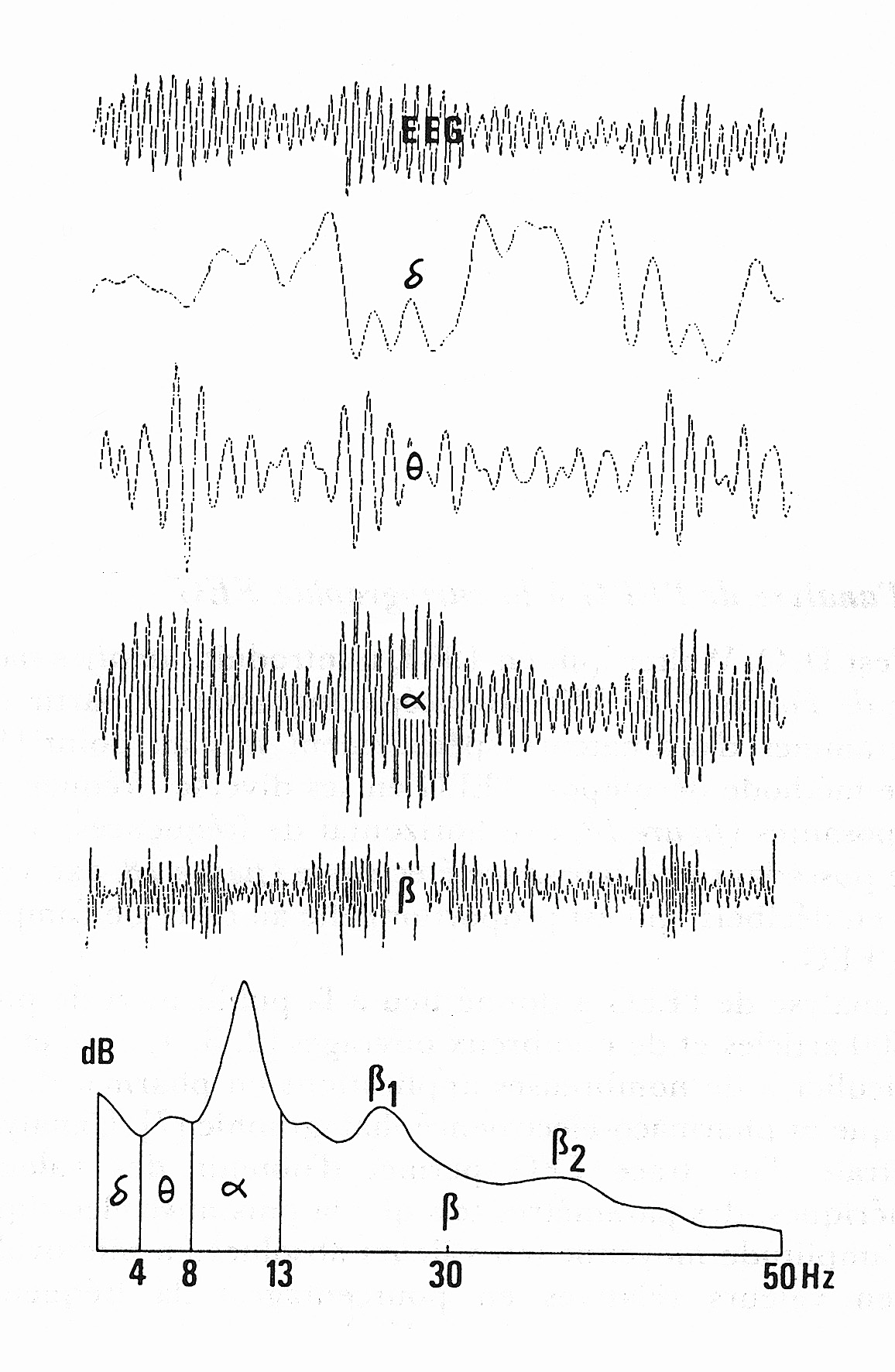
This chart shows a decomposition of the overall electrical activity (top), into its constituent frequency bands. The bottom chart shows these bands on the x axis, along with their respective band power on the y axis. It turns out that lower frequencies (\(\theta, \alpha\)) tend to be associated with states of sleep or relaxation, while higher frequencies (\(\beta\)) are involved with cognitive tasks. By looking at single frequency bands–or combinations of frequency bands–we can get an idea of a person’s mental state. Here are a few recipes for useful frequency ranges/combinations. These metrics are based on band power, or strength of the signal, in the frequency range of interest. Note several of these are courtesy of the MuseLSL neurofeedback script.
Alpha band power: This method simply returns the \(\alpha\) band power, which is an index of degree of relaxation. Here, higher alpha means more relaxation, and possibly fatigue.
Beta Protocol: This is a broad index of mental activity/concentration, and is defined as \(\beta / \theta\) band power. Higher beta can be interpreted as more concentration.
Fatigue: This method captures degree of fatigue, and is calculated as \((\theta + \alpha) / \beta\). An increase in this metric reflects more fatigue.
These metrics are easy and simple to compute, meaning that they are great options for our simple mental state decoding algorithm. Now that we have a conceptual understanding, it’s time to turn our attention to implementing it. I will discuss the process generally while also including code snippits based on a 2014 headband connection. To get a full picture of how the code is working, see here. At a high level, given our continuously streaming EEG data, we want to output a numerical estimate of our above measures (a number between zero to one, for example). Here are some simple steps to achieve this.
Buffering the signal
The sampling rate of the Muse headband can vary, but regardless we will need a way to buffer incoming data so that we can compute frequency bands on the incoming signal. A longer data buffer will make our environment less responsive, but will also make our analysis more robust when it comes time to average the signal. Selecting overlapping buffers can help keep the environment responsive while also keeping a long enough window to average over. Incoming data can easily be stored in a Python NumPy array as the buffer.
Computing spectral powers
Once we have buffered data, we need to compute power spectra. Though we could do this using a fast Fourier transform, Muse provides real-time computed estimates of all the band powers we will need. Make sure to use the absolute band powers if you use the Muse-provided calculations, as the relative will give each frequency band power as a proportion of the total across the full full range.
Note that if you opt to use the Muse-computed spectral powers, steps 1 and 2 can be combined by simply buffering the provided frequency estimates.
We can set up a buffer to track incoming data by:
1
2
3
4
5
6
7
8
9
10
11
12
13
14
15
16
class NeuroFeedback(object):
    """Code to compute basic neurofeedback measures"""
    def __init__(self, bufferWindowSize, minMaxWindowSize,  out_q):
        self.bufferWindowSize = bufferWindowSize
        self.minMaxWindowSize = minMaxWindowSize

        #Create buffer to average down high frequency updates that looks bufferWindowSize into the past
        keys = ['alpha', 'delta', 'beta', 'theta']
        update_keys = ['alpha-relaxation', 'beta-concentration', 'fatigue']

        self.abs_spectrum_powers = dict(zip(keys, [np.zeros(200) for i in range(len(keys))]))
        self.buffer_spectrum_ixs = dict(zip(keys, [0]*len(keys)))

        #Create buffer for rolling min-max storage that looks minMaxWindowSize into the past
        self.rolling_min_maxs = dict(zip(update_keys, [np.zeros(self.minMaxWindowSize) for i in range(len(keys))]))
        self.rolling_min_max_ixs = dict(zip(update_keys, [0]*len(keys)))
Then, each time an async OSC update fires, populating the buffer with the most recently received value:
1
2
3
def abs_frequency_update(self, spectrum, value):
   self.abs_spectrum_powers[spectrum][self.buffer_spectrum_ixs[spectrum]] = value
   self.buffer_spectrum_ixs[spectrum] += 1
Averaging
Now that we have a buffer of values for each frequency range, it is helpful to average over our buffer. This makes our algorithm robust to noise over the interval to give us a more accurate estimate of band power during this time period.
1
2
3
4
5
6
7
8
9
10
11
def compute_power_updates(self):
   '''Take average over the cached buffer'''
   power_updates = {}
   for key in self.buffer_spectrum_ixs.keys():
      power_updates[key] = np.sum(self.abs_spectrum_powers[key]) /\
            np.count_nonzero(self.abs_spectrum_powers[key])

      self.buffer_spectrum_ixs[key] = 0
      self.abs_spectrum_powers[key].fill(0)

   return power_updates
Computing the mental state metrics
Now it is time to compute the actual neurofeedback metrics we talked about above–a matter of simple arithmetic according to the equations. Voila–we now have a number corresponding to relaxation, concentration, and fatigue!
1
2
3
4
update = {}
update['alpha-relaxation'] = power_updates['alpha']
update['beta-concentration'] = power_updates['beta'] / power_updates['theta']
update['fatigue'] = (power_updates['theta'] + power_updates['alpha']) / power_updates['beta']
But, you may be thinking, there is an issue. In fact, there is no guarantee that these values will range within zero to one, or any fixed interval for that matter.
This is important to address since we’ll need a number, say from zero to one, which reflects the mental state we are interested in. We could use min-max standardization such that:
\[z_i=\frac{x_i-\min(x)}{\max(x)-\min(x)}\]which would work, but also poses a problem. Specifically, we can’t know the minimum and maximum values we are going to observe ahead of time. Even if we could know these values, we don’t necessarily want to use them. This is because though we could guarantee that our metrics will fit in a standardized range, they may not actually vary much. We could set our minimum and maximum values based on the most and least relaxed we could possibly be, but most of the time we won’t be in that area, our metrics will float around \(.5\). If our values are normally distributed, this becomes especially problematic.
The real issue arises when we try to pipe our number into an environment–say lights. We would find ourselves in a situation where the lights are not actually changing much in response to changes in mental state.
Though this is a tricky problem, there is a simple solution.
Min-max buffering
If we store the values observed over the last \(N\) buffers, we can compute the current metric based on the minimum and maximum observed over the past \(N\) metric computations. This results in a situation where the sensitivity adapts based on the min-max buffer length. A longer min-max buffer will be less responsive to session changes, but also more stable and reflective of the absolute degree of relaxation / fatigue. This can be implemented by keeping a buffer (NumPy array for example) of recent updates and grabbing the min / max over this buffer.
This approach is also nice because it is relative to the specific user and session (though you could argue this is also a drawback). Yay, now that we have a mental state metric, it is time to hand it off to our environment. This can be done in a number of ways including HTTP or sockets.
1
2
3
4
5
6
7
8
def standardize_updates(self, update):
   '''Standardize update based on min-max standardization,
   where the min and max are calculated dynamically based on recently seen values'''
   for key in update.keys():
      update[key] = (update[key] - np.min(self.rolling_min_maxs[key])) /\
            (np.max(self.rolling_min_maxs[key]) - np.min(self.rolling_min_maxs[key]))

   return update
Testing
Before we talk about that though, you may be wondering: does this actually work? I wanted to know the same thing, so set up an ad hoc experiment to test it out. The experiment? Two minutes learning the general theory of relativity, two minutes relaxing with eyes closed. I first fixed the min-max buffer based on a five minute session to allow for a fair scale comparison under the two conditions, and made sure that my Muse headband was on properly. Unfortunately, I only collected data for the alpha and beta protocols.
Here are the results we get:

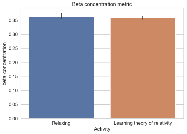
As you can see, the alpha protocol turned out to work quite nicely, while the beta was less-robust. Clearly, this one session is can’t be used to establish anything conclusively, but it at least gives us some assurance that the general approach works. Now that we have a functional metric, we can move on to creating interactive environments.
The environment
I won’t go into any depth about how to create an environment, that is for your own creativity, but I will show a few examples to get the creative juices flowing. Credit for creating the environmental aspects of these projects goes to the teams I worked with, both of which did a beautiful job creating interactive systems.
Breakpoint:
Breakpoint is a programming environment that alerts coders when they are too fatigued to productively code using the fatigue protocol discussed above. The idea is that once fatigue values surpass a threshold for long enough, the programmer gets a notification to take a break. There are plenty of bells and whistles here of questionable utility–but they are pretty cool none-the-less. This project was a hackathon project completed at the Swiss competition, StartHack.
Zenvironment:
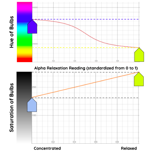
Zenvironment pipes the relaxation value calculated from the alpha protocol into a hue lighting system and sound environment, creating surroundings which ebb and flow based on feelings of calmness. This demo also includes a movement component, which is included as a baseline measure to visualize responsiveness. This project was done as part of my capstone course.
Interestingly, we can also see a concrete way of mapping the relaxation metric to lighting values based on a nonlinear function. The precise function used is up to you, but one that we found works well is:
Wrapping up
That is all, we’ve now built a system that can capture broad user mental states and reflect them in the environment in creative ways. Though this doesn’t include all components of neurofeedback, which typically involves a user leveraging external cues to reach a mental state, it does give a vivid and useful portrait of how a person is feeling. Hopefully now you have the tools to adopt this simple mental state detection process for your next project!